It is useful to know the underlying formula that Xmrit’s free tool implements.
This method to calculate an XmR chart is from Donald Wheeler, who includes the steps in Understanding Variation and in Making Sense of Data.
The Method
Calculating an XmR chart is very simple. We shall use the following data:
| In-process Inventory (100s of Pounds) | Jan | Feb | Mar | Apr | May | Jun | Jul | Aug | Sep | Oct | Nov | Dec |
|---|---|---|---|---|---|---|---|---|---|---|---|---|
| Year One | 19 | 27 | 20 | 16 | 18 | 25 | 22 | 24 | 17 | 25 | 15 | 17 |
| Year Two | 20 | 22 | 19 | 16 | 22 | 19 | 25 | 22 | 18 | 20 | 16 | 17 |
| Year Three | 20 | 15 | 27 | 25 | 17 | 19 | 28 |
- Plot a time series for the metric (X) you’re interested in. In this case In-process Inventory.
- Calculate and then plot the moving range for that same metric. The moving range is simply the difference between two successive data points in the X metric. Note that there should be no negative moving range numbers here — we’re interested in the magnitude differences, not whether the numbers go up or down.
| Moving Range for In-process inventory | Jan | Feb | Mar | Apr | May | Jun | Jul | Aug | Sep | Oct | Nov | Dec |
|---|---|---|---|---|---|---|---|---|---|---|---|---|
| Year One | 8 | 7 | 4 | 2 | 7 | 3 | 2 | 7 | 8 | 10 | 2 | |
| Year Two | 3 | 2 | 3 | 3 | 6 | 3 | 6 | 3 | 4 | 2 | 4 | 1 |
| Year Three | 3 | 5 | 12 | 2 | 8 | 2 | 9 |
- Calculate the average for the business metric and plot the average as a straight line through the time series. In this case the average for In-process Inventory is $20.39$.
- Calculate the average for the moving range and plot the average as a straight line through the moving range time series. In this case the average for the moving range is $4.7$.
You’re going to end up with two charts that look like this:
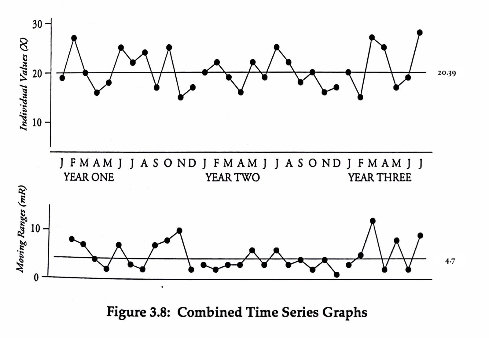
Next, we’re going to calculate the Upper Natural Process Limit (UNPL), the Lower Natural Process Limit (LNPL), and the Upper Range Limit (URL).
- To calculate the UNPL, multiply the average of the moving range by a scaling factor 2.66 and add the product to the average X. $UNPL = Average\ X + 2.66\ Average\ mR$, or $20.39 + (2.66 \times 4.7) = 32.89$
- To calculate the Lower Natural Process Limit: subtract the 2.66 x mR product from the average of X. $LNPL = Average\ X - 2.66\ Average\ mR$, or $20.39 - (2.66 \times 4.7) = 7.89$
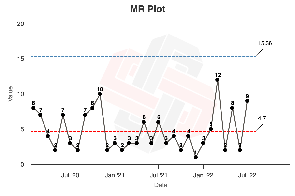
- Finally, calculate the Upper Range Limit (the upper limit for the moving range) by multiplying the average moving range by the scaling factor 3.268: $URL = 3.268\ Average\ mR$, or $3.268 \times 4.7 = 15.36$
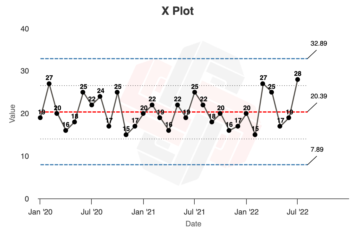
You’ll end up with your final XmR chart, like so (chart):
Donald Wheeler’s Example
The data and example above is taken from Donald Wheeler’s Understanding Variation.
The example in the book is a little different. Wheeler describes a company observing a ‘huge’ (47%) increase in In-process Inventory: this is the change from June (19,000 pounds) to July (28,000 pounds) in Year Three of the data set above. The manager wants to know if such a change is exceptional, or if it’s just ‘business as usual’.
Wheeler does something different. He uses just the first 24 months of data, from Year One to Year Two, to calculate the average lines and limit lines. The reasoning here is that the first two years of data appears to be a stable process; we want to know if the process behaviour in Year Three has changed.
Notice how there is some judgment involved in using XmR charts.
The calculation proceeds as follows:
- We get the average of the first 24 months: this is $20.04$.
- We get the average of the moving range of the first 24 months, this is $4.35$.
- $UNPL = 20.04 + (2.66 \times 4.35) = 31.61$
- $LNPL = 20.04 - (2.66 \times 4.35) = 8.48$
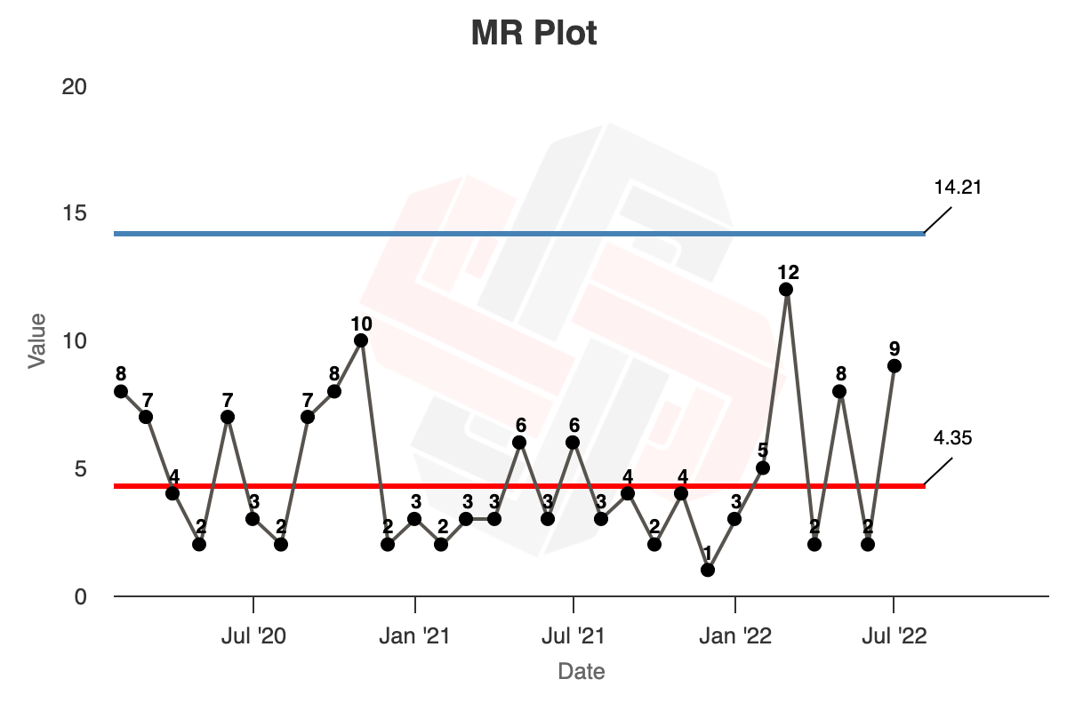
- $URL = 3.268 \times 4.35 = 14.21$
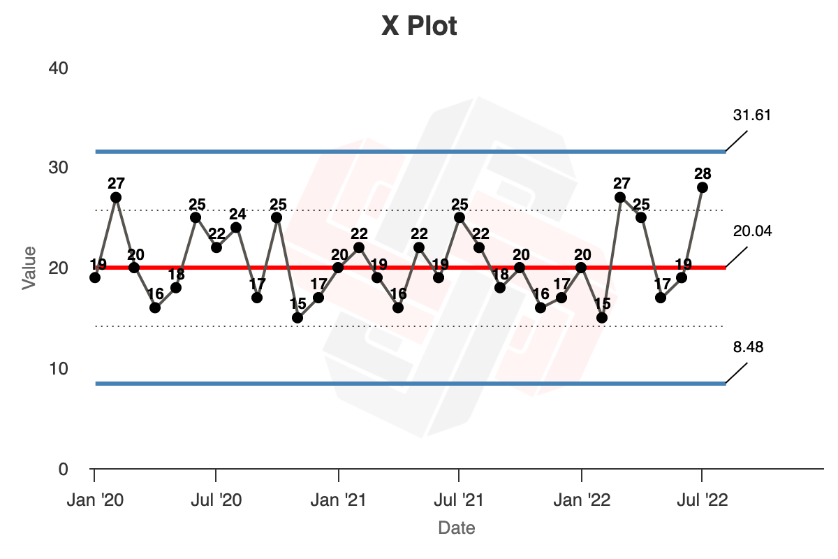
In Xmrit, we may use the ‘Lock Limits’ feature to calculate this chart, as demonstrated here. The rendered charts are as follows:
Where Do The Scaling Constants Come From?
The limit lines in an XmR chart estimate three standard deviations around the average line. However, we cannot use the global standard deviation formula (the one that most of us learnt in high school!) to calculate three standard deviations. We must use a roundabout method to calculate these lines — this is the moving range method that we’ve just discussed above.
Why are we doing such an unusual thing?
The answer is a little involved.
What the XmR chart really is is that it’s a test for homogeneity (which is defined here as a test for whether all the data in a data set are independently and identically distributed). The intuitive way of thinking about this is that it tells you if the variation in a metric comes from one probability distribution, or from multiple probability distributions. (If you’d like more on this, read the Xmrit about page here).
It would be nice if we could just use the global standard deviation formula. However, that formula does the simple thing of characterising the observed variation in your data set. If your data is not homogenous (meaning there may be extreme values as the result of additional probability distributions present), the resulting standard deviation calculation will give you a value that is too large, and therefore will result in limit lines that are too wide. It is for this reason that some publications suggest drawing limit lines around 2.5 standard deviations, calculated using the global standard deviation formula, to cater for this ’too wide’ problem.
This is not ideal, however. The reason we want to estimate three standard deviation is due to Chebyshev’s Inequality, which tells us that no more than 11% of samples from any probability distribution will fall outside of three standard deviations. More importantly, statistician Walter Shewhart (who came up with these charts in the first place) observed that three standard deviations is empirically very useful: while 11% may be the worst case, for many real world distributions you will encounter the percentage of samples falling outside of three standard deviations is between 2-3%. This is wonderful: it means that the risk of a false alarm is around 2-3% for most business metrics you will observe.
So: we want to estimate three standard deviations, but we can’t use the straightforward standard deviation calculation. What do we do?
Enter the ‘moving range’ method, which is properly known as ’the method of successive differences’. This idea was first introduced in a 1941 paper by John von Neumann and three researchers (Kent, Bellinson and Hart) from Aberdeen Proving Ground. The paper describes a method to use successive differences to estimate dispersion. That is to say: we can use the differences between each data point to estimate three standard deviation; it turns out this method is less sensitive to large values if the data is not homogenous (source).
The key relationship we are exploiting here is that the mean value of the successive differences is roughly 1.128 times larger than the standard deviation. Therefore, we have the following formulas:
$ \sigma = \frac{\overline{mR}}{1.128} $
So to get three standard deviation:
$ 3\sigma = \frac{3}{1.128}\ \overline{mR} = 2.66\ \overline{mR} $