XmR chart limits are designed to tell you if your data is exceptional. If your data point is outside your limits that is a sign something has happened in your process that you should investigate. If your data point lies inside your limits you should treat it as routine, and not react to it.
But calculating XmR chart process limits the first time is a confusing process.
Why can we multiply a constant against the average of the moving range and get 3σ process limits? We are usually just told not to worry about it, and just use the constants as provided from the tried and tested scaling constants tables.
But for many of us being told to use something, without an understanding of where it comes from, is uncomfortable. In this article I will show you that the scaling constants are a natural property of your process. Since Xmrit is for operators — not data experts — we will use a spreadsheet simulation to show how you can generate the scaling constants yourself.
The inspiration for this post was from Kenith Grey at r-bar.net, who wrote two posts (1, 2) on deriving XmR chart constants. For those of you who are keen to go deeper into the mathematics behind scaling constants I can recommend Kenith’s work.
3 Sigma (3σ) Limits - Estimating Standard Deviation Using Successive Differences
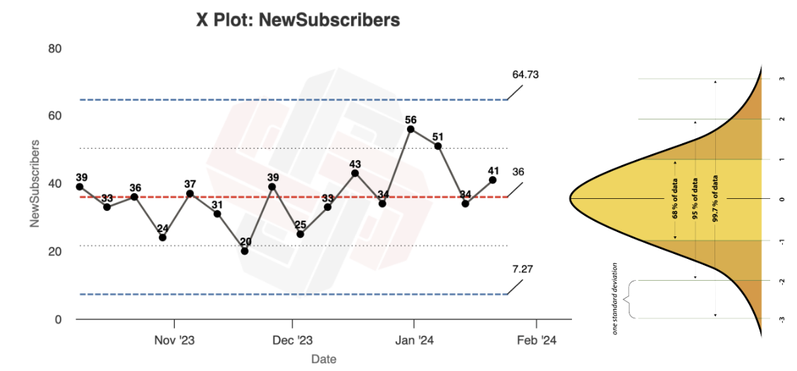
The purpose of process limits is to detect unpredictable variation that has an identifiable cause, known as exceptional variation. We want routine variation to fall within our process limits, and exceptional variation to fall outside of our process limits. We need our limits to strike a balance between not being so wide that only the most extreme exceptional variation is detected, and not so narrow that routine variation is regularly misidentified as exceptional variation.
Through decades of practical use people have found that setting process limits at three standard deviations (3σ) strikes the right balance. In a perfect normal distribution world only 0.3% of our routine variation would be misidentified as exceptional variation.
In Xmrit’s original article on how to build 3σ XmR chart process limits, we used two equations containing three elements; the Process Average (X̅), Moving Range Average (M͞R), and Scaling Constants.
Equation 1: X Chart Process Limit = X̅ +/- (2.660 × M͞R)
Equation 2: MR Chart Process Limit = M͞R × 3.268
X̅ being there is easy to understand, as standard deviations are always measured from the average of a dataset. But instead of directly calculating the σ of the process we use M͞R and scaling constants - why?
The problem is directly using the standard deviation can lead to your process limits being far too wide, hiding exceptional variation. This happens because the direct standard deviation calculation is overly sensitive when exceptional variation is present. Using the average of the moving range and scaling constants is a method to estimate the standard deviation, without the process limits being overly biased by exceptional variation.
At Xmrit we highlight the benefit of the successive differences method every time you use the tool. Our pre-populated standard graph, an example from Dr. Wheeler, has obvious exceptional variation on its final datapoint. This exceptional point is detected with process limits generated using the successive differences method. But if you create process limits based on the standard deviation of this data the limits are so wide that no exceptional variation is detected.
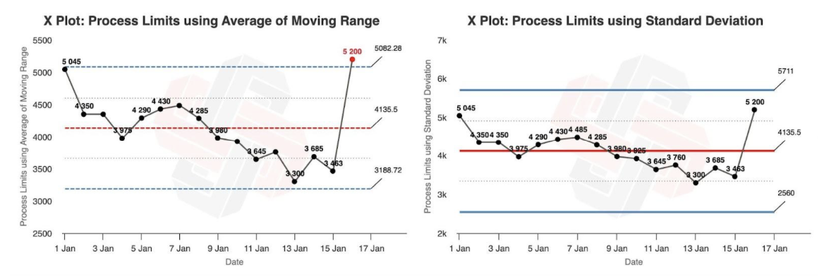
Link to successive differences process limits- Link to Standard Deviation process limits
Estimating the standard deviation via a moving range is called the successive differences estimate of dispersion, or the successive differences method. Wheeler believes it was first developed for field artillery calculations in the late 1800s, but was first written about in the scientific literature in a 1941 article by Von Neumann.
But why does the successive differences method work, and why do we need to use specific scaling constants? In the next section, using only a spreadsheet and a little algebra, I will prove to you that:
- The successive differences method is a reliable way to estimate the standard deviation of a dataset.
- Why the 3σ scaling constants, 2.660 and 3.268, are natural properties of data, and show you how to generate them yourself.
Generating XmR Scaling Constants From 10,000 Random Numbers
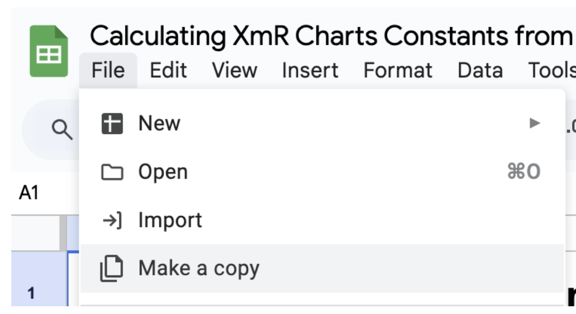
This section will use the following spreadsheet for the simulation. If you would like to refresh the simulation with new values make a copy by clicking File in the top left corner and selecting Make a Copy (you will need to be logged into Google to make a copy). Every time you edit the spreadsheet the simulation will be refreshed with new numbers.
The simulation file consists of three sections:
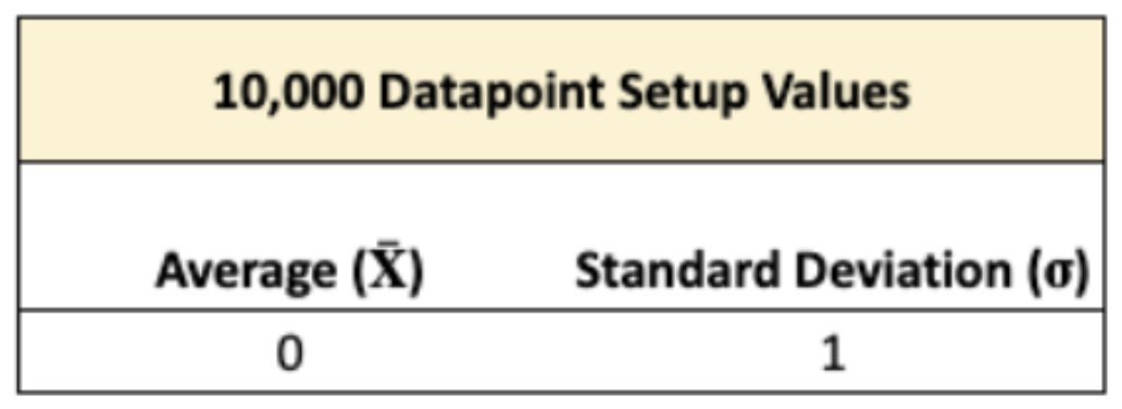
- Setup values for the simulation
- The simulation of 10,000 random data points, and the moving range for those data points.
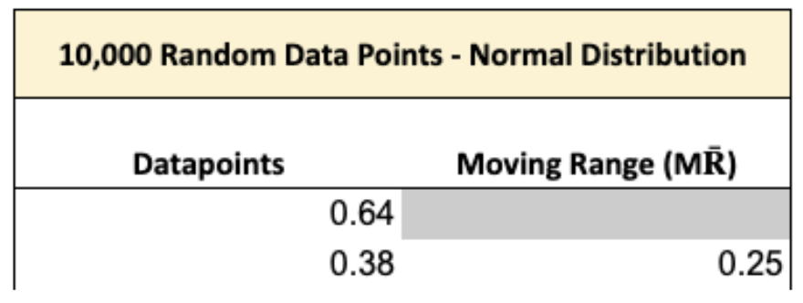
- Comparison of the estimated 3σ limits against the “True” 3σ limits for the X and MR charts.
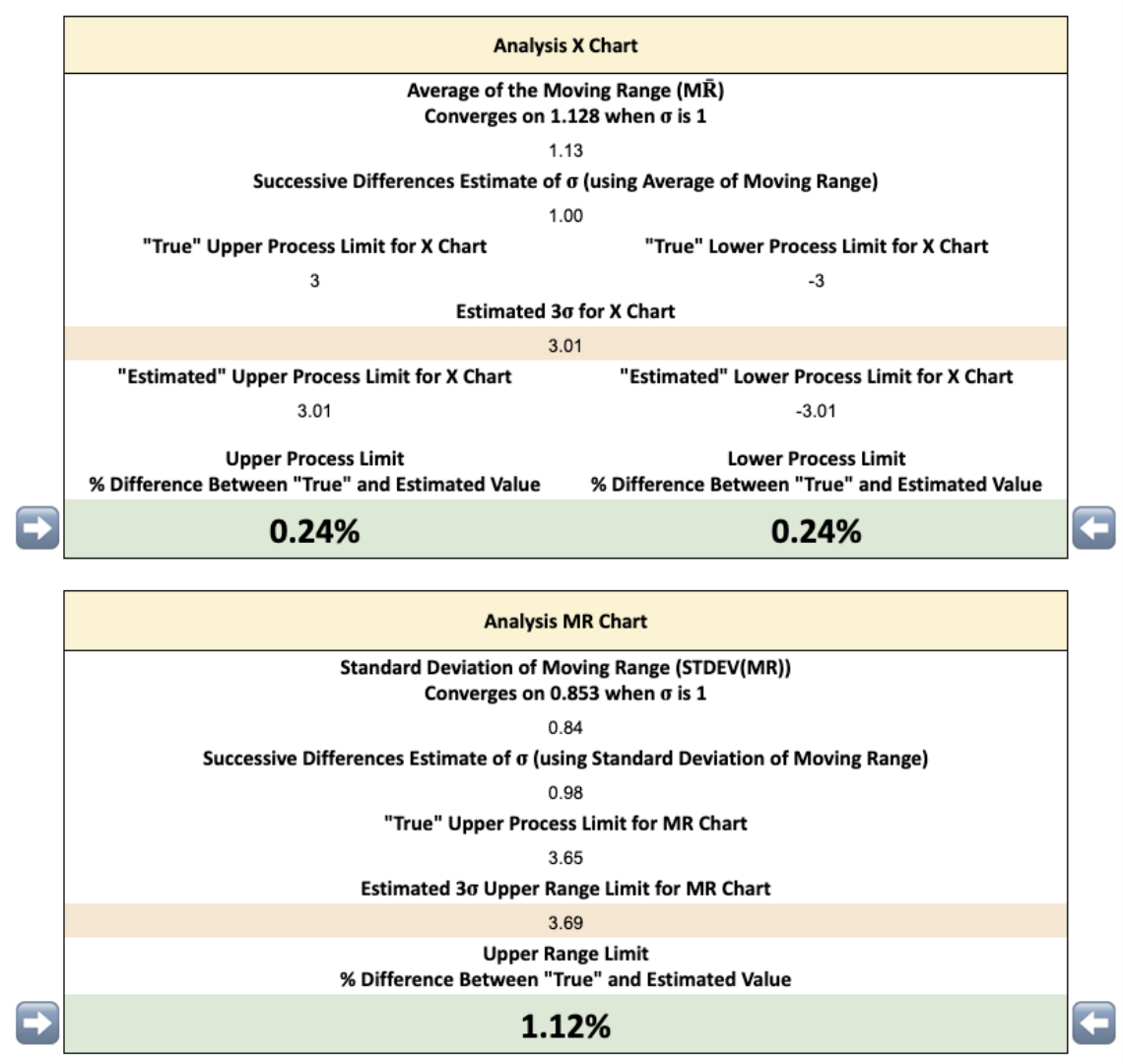
Using these 10,000 random numbers we will be able to see how the successive differences method accurately estimates the standard deviation, and where the scaling constants come from.
Simulation Setup Values
To make the maths for the simulation analysis super simple we have to make three setup assumptions about the 10,000 random numbers.
- Normal: We want to make our random numbers follow a normal distribution. This is specified by the NORMINV(RAND()) that generates the values in the data points column.
- X̅ = 0: The 10,000 random numbers should have an average of 0. You can find and edit this assumption in the setup section.
- σ = 1: The 10,000 random numbers should have a σ of 1. You can find and edit this assumption in the setup section.
Generating X Chart Scaling Constants From the Simulation - 1.128 & 2.660
X Chart: σ = 1 and X̅ = 0
Starting with the X chart we need to go from 10,000 random numbers to the scaling constant of 2.660.
The first step is to calculate the average of the moving range data. When you do this you will notice that despite the numbers being randomly generated no matter how many times you refresh the simulation you always end up with a number close to 1.128.

This is an important finding, as it shows there is a stable relationship between the average of the moving range and the standard deviation (σ). Since we set σ as 1 we can express this relationship as:
Equation 3: σ = M͞R/1.128
To go from this relationship to calculating 3σ limits only requires us to multiply the above equation by 3.
Equation 4: 3σ = (3/1.128) × M͞R
Finally to generate 3σ limits you just need to set the centre of the limits to be +/- the X̅.
Equation 5: 3σ Limits = X̅ +/- (3/1.128) × M͞R
One further simplification and we can generate our scaling constant of 2.660
Equation 6: 3σ Limits = X̅ +/- (2.660× M͞R)
To validate the scaling constant works we will calculate the estimated 3σ limits. Since we set our simulation up with a Standard deviation of 1 we are expecting our 3σ limits to be equal to 3 - and that is what we find!
Equation 7: 3σ Limits = 0 +/- (2.660 × 1.128) = +/-3.00
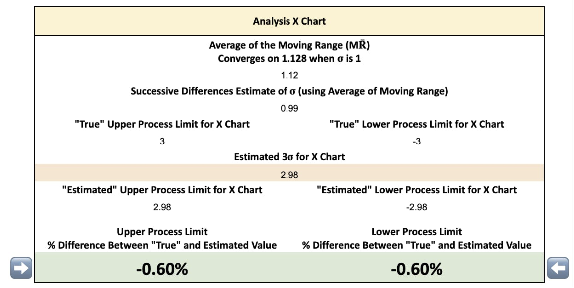
Of course the average of our moving range is not perfectly 1.128 each time we refresh the simulation. This leads to a small % difference between the “True” 3σ limits and the ones generated by the simulation. But thanks to the simulation having a large number of datapoints we usually end up within 2% of the “True” value.
But what if we set our simulation with a different X̅ and σ, would it still work? The answer is yes, it does not matter what the setup average and σ you will always end up with estimated 3σ limits close to the “True” values. Let’s have a look at a couple of examples to demonstrate this, but you can also experiment yourself by editing the simulation.
X Chart: σ = 2 and X̅ = 0
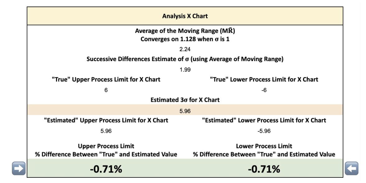
If your setup values are with an X̅ of 0 and a σ of 2 the 3σ limits should be +/-6.
As you refresh the simulation you will find the M͞R is always close to 2.256 - which is 2 x 1.128. When we enter 2.256 into the equation we find our 3σ limits of +/- 6.
Equation 8: 3σ Limits = 0 +/- (2.660 × 2.256) = +/-6.00
X Chart: σ = 3 and X̅ = 1
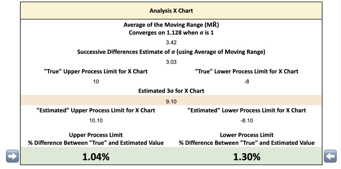
If your setup values are with an X̅ of 1 and a σ of 3 the 3σ limits would now be symmetrical around the X̅ of 1, and would appear at 10 and -8.
As you refresh the simulation you will find the M͞R is always close to 3.384 - which is 3 x 1.128. When we enter our X̅ of 1 and our M͞R of 3.384 into the equation we find our 3σ limits of 10 and -8.
Equation 9: Upper 3σ Limit = 1 + (2.660 × 3.384) = 10
Equation 10: Lower 3σ Limits = 1 - (2.660 × 3.384) = -8
Generating MR Chart Scaling Constants From the Simulation - 0.853 and 3.268
MR Chart: σ = 1 and X̅ = 0
The method for generating the upper range limit (URL) constant of 3.268 is similar, but needs slightly different calculations.
The first step is to calculate the standard deviation of the moving range, instead of the average we used for the X chart. The reason for this is the MR chart’s purpose is to detect when the change between two points is exceptional, not if the absolute value of the point is.
When we calculate the standard deviation of the moving range we again find that no matter how many times you refresh the simulation you end up with a value close to 0.853.

Using the same logic as the X Chart example we can now leverage the fact that there is a constant relationship between the standard deviation of the moving range and σ to generate the following equation.
Equation 11: STDEV(MR) = 0.853σ
Using equation 3 from our X chart calculation we can replace σ:
Equation 12: STDEV(MR) = (0.853/1.128) × M͞R
Now to calculate 3 standard deviations of the moving range we multiply both sides by 3
Equation 13: 3× STDEV(MR) = ((3 × 0.853)/1.128) × M͞R
To calculate the Upper Range Limit (URL) we set it to be 3 standard deviations from the average of the moving range.
Equation 14: URL = M͞R + 3 × STDEV(MR)
We then substitute in equation 13 for the standard deviation of the moving range, and multiply it by 3.
Equation 15: URL = M͞R + (3 × 0.853/1.128) × M͞R
Through the power of factorisation we can reduce this equation to:
Equation 16: URL = M͞R × (1 + ((3 × 0.853)/1.128))
One further simplification and we get to our theoretical scaling constant of 3.268.
Equation 17: URL= M͞R × 3.268
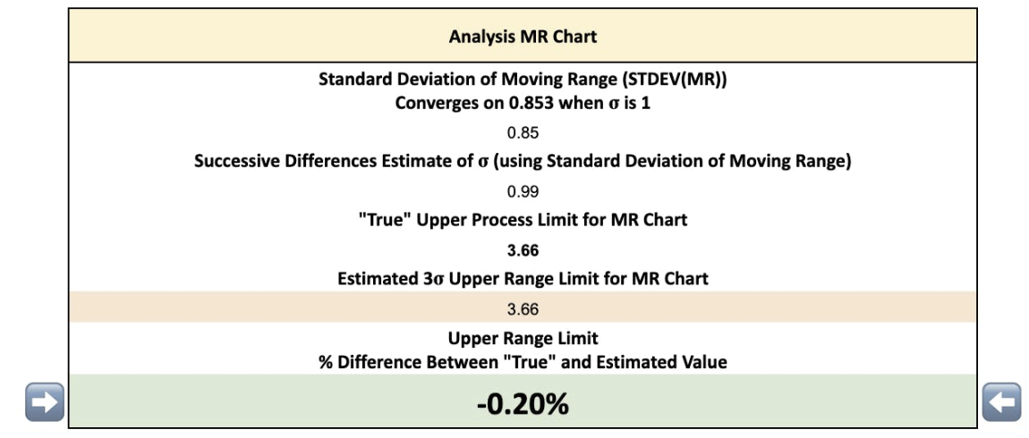
The STDEV(MR) in the simulation will not always be perfectly 0.853. But, just like with the X chart, thanks to the simulation having a large number of datapoints we usually end up within 2% of the “True” value.
It is also possible to edit the simulation setup inputs, and validate that the estimation process works for various values.
MR Chart: σ = 2 and X̅ = 0
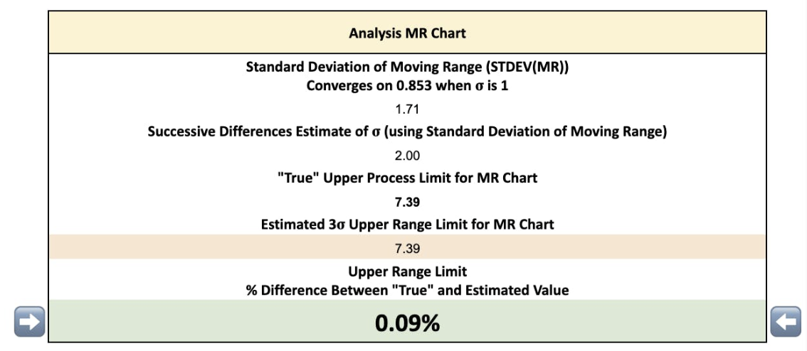
If your setup values are an X̅ of 0 and a σ = 2 the STDEV(MR) will converge to 1.701 - which is 2 × 0.853. You can validate this does happen by refreshing the simulation.
MR Chart: σ = 3 and X̅ = 1
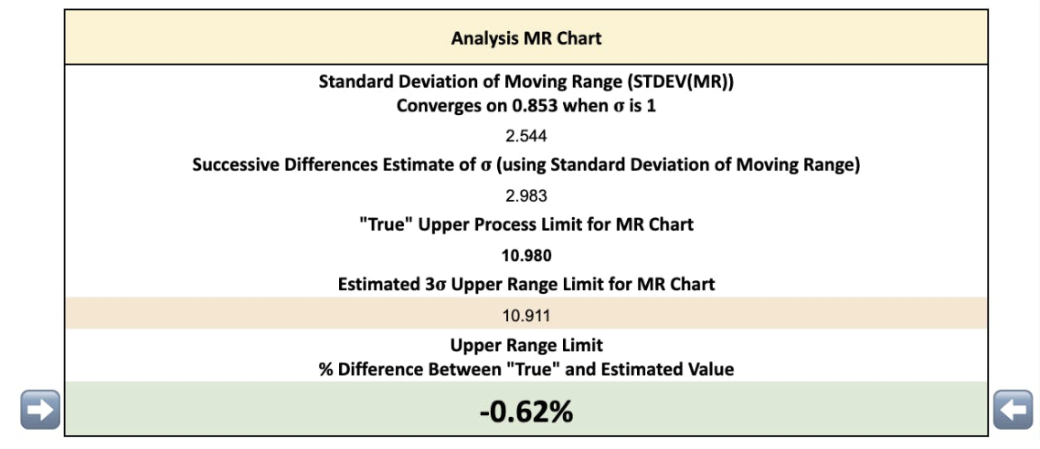
Unlike with the X chart changing X̅ does not impact the MR chart upper range limit.
Therefore, since σ = 3 the STDEV(MR) will converge to 2.559 (3 × 0.853). You can validate this does happen by refreshing the simulation.
Summary
As business operators we are interested in tools and solutions that work. XmR charts have been used and tested for 80+ years, and have repeatedly proven themselves as one of the simplest ways to identify exceptional variation in your processes. But being told to use a tool without understanding how it works can reduce confidence in even the best tools.
In the simulation discussed in this article we saw that the constants of 1.128 and 0.853 are a natural property of datasets, which then turn into our scaling constants of 2.660 and 3.268. Importantly by the simulation being in a spreadsheet it is easy to verify and understand, even for non-technical operators.
If you want to go further into the mathematics of control chart constants I recommend Kenith Grey’s work at r-bar.net as a starting point. You can also read Dr. Wheeler’s more advanced books such as Normality and the Process Control chart and Advanced topics in Process Control Charts.
Going deep into the mathematics and history of control charts is interesting, but not required. You can get the benefit of using XmR charts without having to know their statistical underpinnings.
In the next section I run through some common questions that people have on the simulation.
FAQ
We used a normal distribution for the simulation, what about non-normal distributions?
In our simulation we used a normal distribution to generate the 10,000 random numbers. Many processes have a probability distribution that closely matches a normal distribution, but not all. It is a fair question to ask how well do the scaling constants stand up to non normal distributions?
The answer we give at Xmrit is yes, you can use your XmR charts without having to worry too much about the distribution of your data. For the vast majority of distributions you will encounter the scaling constants for standard charts will work, and in the instances they don’t there are obvious visual cues and solutions to the challenge. The full list of edge cases and solutions is covered in detail of Module 1 of the Metrics Masterclass.
But the normal distribution question is a longstanding debate in the control chart space. Theoretically-minded textbooks, like Introduction to Statistical Quality Control by Douglas C. Montgomery (6th edition), emphasises that once your process only has routine variation that the risk of false alarms of exceptional variation becomes a problem. In response Dr. Wheeler has written numerous articles arguing that this view is mistaken (1, 2, 3, 4) and even an entire book on the topic, Normality and the Process Behaviour Chart.
After using XmR charts on Commoncog and Xmrit data we have come to agree with Dr. Wheeler. XmR charts are robust to the wide range of data you will find in your business. And in the situations where it does not work it is quickly obvious, and there are standard fixes you can implement.
We used 10,000 data points for the simulation, how good are the estimates for smaller datasets?
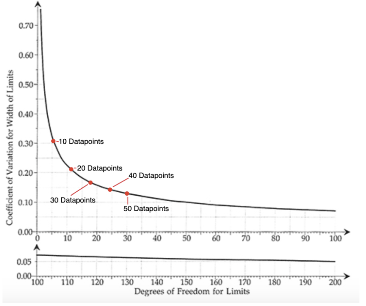
The fewer data points you have the greater the uncertainty you will have in your process limits. In Xmrit’s article on locking limits we showed how the uncertainty drops as you use more data. The simulation purposely used a large number of datapoints to get the final estimate close to the theoretical scaling constant values.
The successive differences method is influenced less by exceptional variation. Is there anything even less influenced by exceptional variation than it?
If you want a method for estimating 3σ limits that is even less influenced by exceptional variation the recommended method is to use the median moving range instead of the average moving range.
Since medians are less impacted by outliers than averages it is less influenced by exceptional variation. However, the scaling constants used for the median moving range are different (and can be derived the same way that was done for the average moving range simulation):
Process limit = X̅ +/- 3.145 × median(MR)
MR URL = median(MR) × 3.865
Generally the average method gives better estimates of the standard deviation than the median method, but the median is a great way to deal with data that you believe has a lot of exceptional variation in it.
